This is a blog to demystify encoders in Large Language Model (LLM) transformers as applied to genomics via a simplified gap-aware sequence transformer named ShallowConsensus.
In the previous blog we applied the concepts of a neural network to genomics via a variant caller named ShallowVariant. Here we will build a simpler variation of Google’s DeepConsensus using an encoder-only transformer, to illustrate a practical example in the area of Genomics with Machine Learning.
Our Goal
Sometimes when a sequencer provides reads, we might have gaps between the sequences out of which we want to build a consensus sequence (such as de novo sequence assembly). We want to train a transformer (encoder-only) to be able to take such sequences, and fill in the gaps correctly. Our approach should be much smaller and faster than actually searching the genome for the correct contextual subsequence.
Downloading the Data
The first step is to download the necessary file:
The only file that is necessary is the the sequence of one gene, which in this case is BRCA1 (BReast CAncer gene 1 coding sequence).Homo sapiens isolate OC-10 mutant BRCA1 protein (BRCA1) gene, partial cds: https://www.ncbi.nlm.nih.gov/nuccore/OQ235086.1?report=fasta The program can work and will improve the training with more sequences, but we wanted to keep the example simple.
This file is sufficient to get us started.
What is a Transformer?
The idea of a transformer was first proposed by Vaswani, et. al. in a Google paper called Attention is All you Need mainly for the application of language translation. The transformer architecture is core to ChatGPT, but has emerged to have useful properties that can be applied to other fields as well, such as genomics (where DNA is both a language and a vocabulary). The general architecture is the following:
Figure 1: The transformer architecture showing the encoder and decoder.
Before diving into the transformer architecture, it provides three major benefits over the previous approach in machine translation (Recurrent Neural Networks):
Transformers are highly parallelizable.
Transformers work well with long sequences.
Transformers are able to capture context (affinity) among words in a sentence, through a method called attention.
The high level view of a transformer is the following:
The Encoder learns a language from two elements:
The vocabulary of a language.
The affinities of words to other words based on sentences from a corpus.
Based on these it is able to be given a sentence, and predict the next word in the sentence.
The Decoder is trained in a similar way, but it is trained so that the correct predicted word from the Encoder is the same one in a translated language.
Let us dive a little bit deeper in the Encoder, as the Decoder has a similar design and for our implementation of ShallowConsensus we only need the Encoder for now.
Embedding the Vocabulary
Computers prefer to work with numbers, especially when performing any mathematical analysis across a dataset. In our case we will be using DNA to encode them as numbers, and with only 4 bases (A, T, G and C) sliced at different short subsequence lengths this should be more trivial than the vocabulary of the English language. These come in the form of a vector of any desirable size, where each word (base or subsequence) becomes encoded as an unique series of numbers representing it. Thus a matrix of such vectors becomes the word embedding of a vocabulary. These numbers can change as the training is performed and words that display close association with each other, will have a similar vector direction (or cosine similarity).
Let’s start with how we used our gene (BRCA1) to begin coding the Encoder. I will jump into code as soon as one aspect is covered and continue going back-and-forth to illustrate the practical application of the theory.
# Here we used a file called genome.txt to store our BRCA1 sequence
\$ cat genome.txt
GGTGTCCACCCAATTGTGGTTGTGCAGCCAGATGCCTGGACAGAGGACAATGGCTTCCATGCAATTGGGC
AGATGTGTGAGGCACCTGTGGTGACCCGAGAGTGGGTGTTGGATAG
\$
Since the encoder $\text{–}$ just like a human $\text{–}$ will be able to learn better with more text, we will provide multiple copies of the BRCA1 sequence in the genome.txt file. That will look something like this $\text{–}$ though a more reprentative approach would be the sequence of the whole genome:
# Here we used a file called genome.txt to store our BRCA1 sequence
\$ cat genome.txt
GGTGTCCACCCAATTGTGGTTGTGCAGCCAGATGCCTGGACAGAGGACAATGGCTTCCATGCAATTGGGC
AGATGTGTGAGGCACCTGTGGTGACCCGAGAGTGGGTGTTGGATAG
GGTGTCCACCCAATTGTGGTTGTGCAGCCAGATGCCTGGACAGAGGACAATGGCTTCCATGCAATTGGGC
AGATGTGTGAGGCACCTGTGGTGACCCGAGAGTGGGTGTTGGATAG
GGTGTCCACCCAATTGTGGTTGTGCAGCCAGATGCCTGGACAGAGGACAATGGCTTCCATGCAATTGGGC
AGATGTGTGAGGCACCTGTGGTGACCCGAGAGTGGGTGTTGGATAG
GGTGTCCACCCAATTGTGGTTGTGCAGCCAGATGCCTGGACAGAGGACAATGGCTTCCATGCAATTGGGC
AGATGTGTGAGGCACCTGTGGTGACCCGAGAGTGGGTGTTGGATAG
...
\$
Next we will load the data into Python as follows $\text{–}$ where again we will be using PyTorch:
# This will be populated with the genomic sequences
genome = ''
# Loading in the gene sequence
with open('genome.txt', 'r', encoding='utf-8') as file:
for line in file:
# Removing the newline character from the genome, as it is unnecessary noise
genome = genome + line.replace("\n", "")
def construct_dna_vocabulary( sequence, splice_size ):
subsequences = []
# Shift and also sub-select up to size of the splice_size
for offset in range( 0, splice_size ):
for i in range( offset, len(sequence) ):
subsequences.append( sequence[ i:(i+splice_size) ] )
subsequences.append( sequence[ i:(i+offset) ] )
# Collect only non-empty entries
non_empty_vocabulary_entries = []
for i in subsequences:
if len( i.strip() ) > 0:
non_empty_vocabulary_entries.append( i.strip() )
vocabulary = sorted( list( set( non_empty_vocabulary_entries ) ) )
return vocabulary
# Construct a vocabulary sliced in sizes of 8 letters or less from the BRCA1 gene
GENOME_SPLICE_SIZE = 8
dna_vocabulary = construct_dna_vocabulary( genome, GENOME_SPLICE_SIZE )
dna_vocabulary_length = len( dna_vocabulary )
print("The vocabulary of DNA:")
print( dna_vocabulary )
The output will be as follows:
The vocabulary of DNA:
['A', 'AA', 'AAT', 'AATG', 'AATGG', 'AATGGC', 'AATGGCT', 'AATGGCTT', ... ]
Notice how in this list of our DNA vocabulary, each subsequence would have an index. We can use that to begin converting our sequence to an equivalent numerical sequence of indices, or vice versa. For that we need a few functions, and variables:
def dna_vocabulary_to_index_mapping( vocabulary ):
index = 0
dna_vocabulary_to_index_dictionary = {}
for subsequence in vocabulary:
dna_vocabulary_to_index_dictionary[ subsequence ] = index
index = index + 1
return dna_vocabulary_to_index_dictionary
def index_to_dna_vocabulary_mapping( vocabulary ):
index = 0
index_to_dna_vocabulary_dictionary = {}
for subsequence in vocabulary:
index_to_dna_vocabulary_dictionary[ index ] = subsequence
index = index + 1
return index_to_dna_vocabulary_dictionary
# A dictionary for converting DNA subsequences to indices
dna_vocabulary_to_index_dictionary = dna_vocabulary_to_index_mapping( dna_vocabulary )
# A dictionary for converting indices to DNA subsequences
index_to_dna_vocabulary_dictionary = index_to_dna_vocabulary_mapping( dna_vocabulary )
def encode_sequence_as_indices( sequence, dna_vocabulary_to_index_dictionary, splice_size ):
encoded_sequence = []
for i in range( 0, len(sequence) ):
encoded_sequence.append( dna_vocabulary_to_index_dictionary[ sequence[ i:(i+splice_size) ] ] )
return encoded_sequence
def decode_indices_into_sequence( indices, index_to_dna_vocabulary_dictionary ):
decoded_sequence = ''
for index in range(0, len(indices) ):
decoded_sequence = decoded_sequence + \
index_to_dna_vocabulary_dictionary[ indices[ index ] ]
return decoded_sequence
As before we will need to split our data into a training and testing group, so we might as well do it now, while still dealing with the input data:
# Training and testing splits
TRAINING_SIZE = 0.8
data = torch.tensor( encode_sequence_as_indices( genome,
dna_vocabulary_to_index_dictionary,
GENOME_SPLICE_SIZE ), dtype=torch.long )
last_index_of_training_data = int( TRAINING_SIZE * len( data ) )
training_data = data[ :last_index_of_training_data ]
validation_data = data[ last_index_of_training_data: ]
Now we have enough to continue with the theory. From the architecture of the encoder, we still need to embed the bases and subsequences of DNA into some sort of vector. For that we will be using the nn.Embedding function from PyTorch. This function requires as input the size of the vocabulary, and how long the the vector of each word will be. For that we will define several variables, or hyperparameters:
# Our seed for the random number generator
torch.manual_seed( 999 )
# The number of groups of sequences we want to
# process independently (in parallel)
batch_size = 8
# If we want to predict the next base, what would
# be the minimum sequence length required
sequence_length_required_for_prediction = 32
# The number of training iterations (usually longer
# is better, but this is a simple example)
number_of_training_iterations = 200
# After how many iterations do we want to present
# the loss, so far of the model
iteration_interval_to_print_loss = 10
# The learning rate (you have seen before)
learning_rate = 3e-2
# The number of losses to keep track of
number_of_losses_to_record = 10
# The granularity of how long the vector of the embedding should be
size_of_granularity_of_representation = 16
# Into how many training groups should we split our data, so that
# the model can learn from multiple perspectives about the data.
number_of_multiple_heads = 4
# The number of repeated encoders, as we will stack multiple
# encoders on top of each other to improve the training of
# our model.
number_of_encoder_blocks = 6
# During rounds of training, what percentage of the nodes in the
# neural network can be hidden in order for the others to compensate
# so that overfitting does not occur.
dropout = 0.1
# This is the amount by which the feed forward network should expand by
# during the self-reflecting stage of the encoder
feed_forward_scaled_expansion = 4
With the above variables, the embedding can be defined as follows, though we shall see later where in the code it will reside:
The last step we should consider is the position of each base or subsequence in the indexed embedded sequence while inquiring the encoder. For that we will be adding to each embedding’s vector positions specifically calculated numbers, which we will define as positional encoding. We will come back to this idea later, when we will be implementing it.
For now we will keep going up the encoder stack.
Ask In Order to Learn
Before we get to the next element of the Encoder, we need to understand a bit about how it learns. Imagine you have the following design:
You start with a sequence, which is a series of bases or subsequences
You have two neural networks that you will push this sequence through:
A $Query$ neural network, and
A $Key$ neural network
If you perform the following operation, you will get an output for each base or sliced subsequence covering every position of the sequence:
$Query( Sequence )$ : This will produce an output for all the bases or subsequences
$Key( Sequence )$ : This will produce another output for all the bases or subsequences
Nothing is happening yet, because we have not made them interact with each other, which happens next via a dot-product:
$Query( Sequence ) \cdot Key( Sequence )^T$ : This is the dot product to check for affinities among bases or subsequences. You can think of this as producing a $Sequence \times Sequence$ matrix of interactions. The keys here are transposed.
This dot-product has all bases (or subsequences) check against all other bases (or subsequences) in the sequence. If their interaction is strong (i.e. the multiplication and addition produce a large number), then the relationship between one base (or subsequence) and another is strong, otherwise not. Strong interactions indicate affinities for each other in a data-dependent manner.
Now we have a $|Sequence| \times |Sequence|$ matrix, but what we want is for the sequence to produce us the affinities to across the sequence. For that we generate the following neural network:
$Value( Sequence )$ : This will produce an output for all the bases or subsequences
If we take the previous dot-product ($Q \cdot K^T$), and perform a dot-product with $V$, we get which bases (or subsequence) in this sequence we should pay more attention to as compared to others. This is the attention score! The actual formula is the following:
You will notice that we divide by a square root term ($d_{key}$). That term is the granularity of the key embedding. This prevents the softmax function from becoming saturated with large values. The $softmax$ function is there so that we work in the space of probabilities.
The question you might still ask yourself is why does this work, and maybe how it is being achieved? Keep in mind that these neural networks have weights that are trainable through many iterations:
These weights will be adjusted by the optimizer given how the attention formula is performed. They will maximize based on the expected next word given multiple sequence contexts. The formulas make them interdependent, and the weights is how their interdependence is adjusted to maximize the expected next output. Notice also that the whole corpus is being fed, so this then becomes self-attentive to maximize on the same language.
Attention is specified as an AttentionHead in our code. Each attention head is implemented as follows in our code:
This clearly illustrates how the affinities get adjusted given the input of the sequence. The $key$ and $query$ neural networks take the base (or subsequence) embeddings, and determine just by the dot product which positioned bases (or subsequences) have the closest affinities. That gets propagated into the bases/subsequences attention matrix for the this head, through the dot product with the values. One thing to note regarding our encoder’s prediction behavior is to capture all the sequence information (including future ones). Thus all bases (and subsequences) beyond our input need to be unmasked during training, as relating to the prediction of the next base. With a decoder that is not the case.
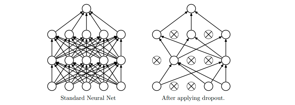
One other element to show here is the dropout function. This comes from a 2014 paper by Srivastava, et al. from the University of Toronto. $Dropout$ is defined as a fraction denoting how many nodes in a network should be hidden in order for the others to compensate. This basically prevents overfitting and will allow the network to become more flexible in capturing the input. Below is a figure from the paper that helps illustrate this idea:
Figure 2: The left figure shows the original network, while on the right is the network after dropout has been applied to some of the nodes.
Let’s keep exploring the attention mechanism.
Attention Observes It All
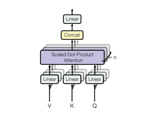
Though it might be natural to have a large corpus and just never split it up, but parallelizing the data into multiple attention blocks, will not only make it faster but also give different perspectives of the data to each attention head. The multi-attention head can be visualized as follows:
Figure 3: The multi-attention head.
Our implementation of this looks as follows:
class MultiHeadedAttention(nn.Module):
""" Multiple heads of self-attention """
def __init__(self, number_of_heads, head_size):
super().__init__()
self.heads = nn.ModuleList([AttentionHead(head_size) for _ in
range(number_of_heads)])
self.proj = nn.Linear( head_size * number_of_heads, \
size_of_granularity_of_representation)
self.dropout = nn.Dropout(dropout)
def forward(self, x):
out = torch.cat([h(x) for h in self.heads], dim=-1)
out = self.dropout(self.proj(out))
return out
Now we have the attention based on the interaction of bases/subsequences given their position in the sequence, thus making it data-dependent. But what if we have something that would reflect upon all these interactions, in order to see if there are more abstract underlying structures in the sequence? This would be something along the lines of an attention brain. This is our next step forward.
The Feed Forward Self-Reflective Brain
Now we will have a feed-forward neural network, where each base (and subsequence) tries to learn something about itself given the attention calculation, thus becoming self-reflective. The code looks like this:
class FeedForward(nn.Module):
""" A self-expansion into a larger neural network with a collapse """
def __init__(self, size_of_granularity_of_representation):
super().__init__()
self.net = nn.Sequential(
nn.Linear( size_of_granularity_of_representation, feed_forward_scaled_expansion *
size_of_granularity_of_representation ),
nn.ReLU(),
nn.Linear( feed_forward_scaled_expansion * size_of_granularity_of_representation,
size_of_granularity_of_representation ),
nn.Dropout( dropout ),
)
def forward( self, x ):
return self.net( x )
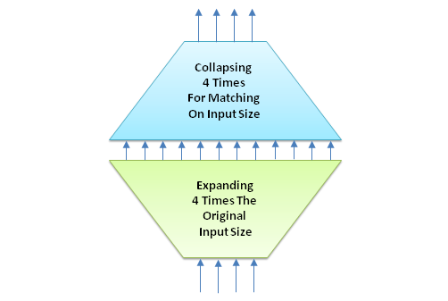
What basically happens here is a neural network expansion of reflecting on the attention of each base or subsequence. The variable feed_forward_scaled_expansion assigned a value of 4 performs this expansion, which can be visualized as follows:
Figure 4: The feed forward network.
Now we have enough that we can put together an encoder block.
The Encoder Block
We are now ready to put it all together, and have implemented it as follows:
All of this I hope will seem straight-forward. We now seem to have two additional nn.LayerNorm functions in our code. All that these perform is to ensure the values do not skew the results, by making sure each batch have a mean of 0, and a variance of 1.
The other important element here is the summation to the original result. These are called residual connections or skip connections, first introduced by Microsoft Research in their paper called Deep Residual Learning for Image Recognition. These skip connections help speed up the optimization process, during back propagation. Initially they contribute minimally $\text{–}$ thus not slowing down the process $\text{–}$ but only later begin to come online as they get more weight during this process.
Now that we have one Encoder block, the process might become even better with more blocks. That is exactly what we will be implementing through our DNAEncoder.
The DNA Encoder
Our initial goal is that given a sequence there is a gap that needs to be filled at the end of it. Thus given a trained model, we would like the gap be filled correctly based on its training data. This should be much smaller and faster than actually searching the genome for the correct contextual subsequence. Thus we want to build a genomic DNA Encoder, with multiple encoder block passes to improve the prediction power. Below is our implementation of it:
class DNAEncoder(nn.Module):
def __init__(self):
super().__init__()
self.dna_embedding_table = nn.Embedding( dna_vocabulary_length,
size_of_granularity_of_representation )
self.encoder_blocks = nn.Sequential(*[EncoderBlock( size_of_granularity_of_representation,
number_of_heads=number_of_multiple_heads) for _ in range(
number_of_encoder_blocks ) ] )
self.layer_normalize = nn.LayerNorm( size_of_granularity_of_representation )
self.project_to_dna_vocabulary = nn.Linear( size_of_granularity_of_representation,
dna_vocabulary_length )
# This helps with the optimizer by presetting the weights
self.apply(self._init_weights)
# This code helps with making the optimizer faster
def _init_weights(self, module):
if isinstance(module, nn.Linear):
torch.nn.init.normal_( module.weight, mean=0.0, std=0.02 )
if module.bias is not None:
torch.nn.init.zeros_( module.bias )
elif isinstance(module, nn.Embedding):
torch.nn.init.normal_( module.weight, mean=0.0, std=0.02 )
def forward( self, sequence_of_indexed_bases_or_subsequences, targets=None ):
BATCHES, QUERY_SEQUENCE_LENGTH = sequence_of_indexed_bases_or_subsequences.shape
sequence_of_embedded_bases_or_subsequences = self.dna_embedding_table(
sequence_of_indexed_bases_or_subsequences )
positional_encoding = torch.zeros( QUERY_SEQUENCE_LENGTH,
size_of_granularity_of_representation )
for query_base_or_subsequence_position in range( 0, QUERY_SEQUENCE_LENGTH ):
for embedding_index in range( 0, size_of_granularity_of_representation ):
denominator = math.pow( 10000,
2 * embedding_index / size_of_granularity_of_representation )
if embedding_index % 2 == 0: # For even base (or subsequence) positions
positional_encoding[query_base_or_subsequence_position][embedding_index] = \
math.sin( query_base_or_subsequence_position / denominator)
else: # For odd base (or subsequence) positions
positional_encoding[query_base_or_subsequence_position][embedding_index] = \
math.cos( query_base_or_subsequence_position / denominator )
positional_embedded_sequence = sequence_of_embedded_bases_or_subsequences + positional_encoding
logits = self.encoder_blocks( positional_embedded_sequence )
logits = self.layer_normalize( logits )
logits = self.project_to_dna_vocabulary( logits )
if targets is None:
loss = None
else:
BATCHES, QUERY_SEQUENCE_LENGTH, DNA_VOCABULARY = logits.shape
logits = logits.view( BATCHES * QUERY_SEQUENCE_LENGTH, DNA_VOCABULARY )
targets = targets.view( BATCHES * QUERY_SEQUENCE_LENGTH )
loss = F.cross_entropy( logits, targets )
return logits, loss
def generate(self, sequence_of_indexed_bases_or_subsequences, max_new_tokens):
for _ in range( max_new_tokens ):
# Here we get the predictions (logits) and loss
logits, loss = self( sequence_of_indexed_bases_or_subsequences )
# The last step is the weighted next probable base
logits = logits[:, -1, :]
# Get the probabilities by applying the softmax
probabilities = F.softmax( logits, dim=-1 )
# Get the 1st most probable next base.
# The multinomial will sample based on that,
# though we chose argmax so as to be more explicit. We commented
# the multinomial approach for reference to the reader
# next_indexed_base = torch.multinomial( probabilities, num_samples=1 )
next_indexed_base = torch.argmax( probabilities ).unsqueeze( dim=0 ).unsqueeze( dim=0 )
# Now append the predicted base index to the running sequence
sequence_of_indexed_bases_or_subsequences = torch.cat( ( sequence_of_indexed_bases,
next_indexed_base ), dim=1 )
return sequence_of_indexed_bases_or_subsequences
You might recognize that we are continuing to use cross-entropy as our loss function. Now besides having multiple encoder blocks for improving prediction power, there is one additional element here that is crucial. We are adding positional encoding to each of the indices, in order to differentiate spatially (temporally) in the sequence, as applied to each base or subsequence. Thus each vector becomes unique. Positional encoding is performed via the following two formulas:
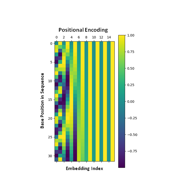
For a short sequence of 32 bases with 16 embedding indices, the positional embedding is the following:
Figure 5: The positional encoding variation given the base position and embedding index.
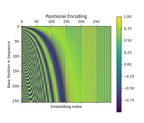
If we increase both the embedding granularity and the length of the sequence, the positional encoding becomes more obvious in its differentiation:
Figure 6: The positional encoding variation given longer sequences with deeper embedding.
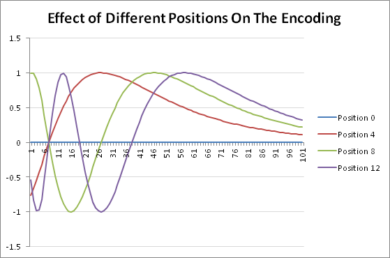
If we look at the contributory effect that position has upon the encoding, this can be clearly seen in the following figure:
Figure 7: The effect of position on the encoding.
The importance provided by positional encoding is that if we have four (4) encoded bases (and additional subsequences) represented as vectors. Without the addition of positional encoding to the embedding, we cannot meaningfully distinguish among them in a sequence. Thus we need a small variation among the vectors to be able to generate slightly diviating new ones that allow us to understand their context in a sequence.
Now we are ready to train a model.
Training the Model
Before training a model we need to add a few helper functions to assist us:
# This function provides a batch of either training or validation data
def get_data_batch_for_processing( training_or_validation_split ):
# Generate a small batch of data of
# inputs x and expected targets y
data = None
if training_or_validation_split == 'training':
data = training_data
else:
data = validation_data
randomly_sample_by_index = torch.randint( len(data) -
sequence_length_required_for_prediction,
(batch_size,) )
x_inputs = torch.stack( [data[ i:(i + sequence_length_required_for_prediction) ] \
for i in randomly_sample_by_index])
y_expected_targets = torch.stack(
[data[ (i + 1):(i + sequence_length_required_for_prediction + 1) ] \
for i in randomly_sample_by_index] )
return x_inputs, y_expected_targets
@torch.no_grad()
def estimate_the_loss():
average_loss = {}
model.eval()
for training_or_validation_split in ['training', 'validation']:
losses = torch.zeros( number_of_losses_to_record )
for k in range( number_of_losses_to_record ):
X, Y = get_data_batch_for_processing( training_or_validation_split )
logits, loss = model( X, Y )
losses[ k ] = loss.item()
average_loss[ training_or_validation_split ] = losses.mean()
model.train()
return average_loss
Now we can begin to create the model and optimizer:
# Our model
model = DNAEncoder()
# Create our optimizer
optimizer = torch.optim.AdamW(model.parameters(), lr=learning_rate)
You will notice that we are using AdamW, where before we used Adam. The only major difference is in the weight decay, otherwise they are the same.
Now we are ready to run through 100 steps (rounds) to train the model, while checking on its loss and validation:
for round_of_iteration in range(number_of_training_iterations + 1):
# After every 10 rounds we display our loss for both
# training and validation datasets
if round_of_iteration % iteration_interval_to_print_loss == 0:
losses = estimate_the_loss()
print( f"After {round_of_iteration} rounds: training loss={losses['training']:.4f}, \
validation loss={losses['validation']:.4f}" )
# Get a batch of data
x_batch, y_batch = get_data_batch_for_processing( 'training' )
# Determine the loss
logits, loss = model( x_batch, y_batch )
# Optimize
optimizer.zero_grad( set_to_none=True )
loss.backward()
optimizer.step()
Below is our training and validation dataset losses:
Round
Training Loss
Validation Loss
0
6.3932
6.3953
10
4.7555
4.7607
20
4.7259
4.7211
30
4.6002
4.6142
40
4.4297
4.4948
50
4.2193
4.2346
60
4.0673
4.1132
70
3.9200
4.0213
80
3.7147
3.7543
90
3.5165
3.4834
100
3.2278
3.1845
110
2.8611
2.8419
120
2.6257
2.6392
130
2.0924
1.9680
140
1.1518
1.2116
150
0.5888
0.6429
160
0.2655
0.2873
170
0.0847
0.0730
180
0.0158
0.0159
190
0.0078
0.0077
200
0.0040
0.0041
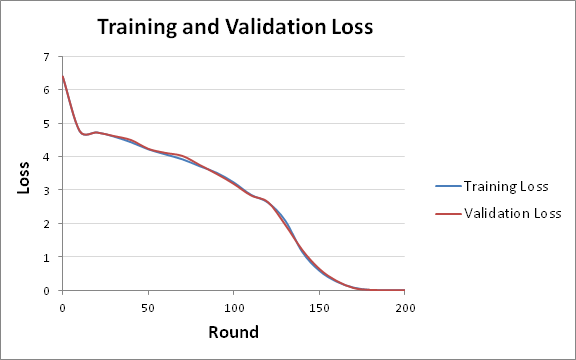
Below is a figure illustrating the training and validation loss over 200 rounds:
Figure 8: The training and validation loss across 200 rounds.
Naturally the losses look good, with a decrease to with each round down to a low loss after 200 rounds. All of these all were performed on a CPU, which took less than 30 seconds, and if a GPU would have been utilized then more rounds could have been processed faster.
Making Some Predictions
Now let us try to predict some bases in a gap. We will want to predict what the bases are in the gap between the two subsequences:
CCACCCAATTGTGGTTGTGCAGCCAGATGCCT--ACAGAGGA
Before we perform the predictions, we will need a couple of helper functions:
# This function will look at a dictionary of bases::base_counts for picking
# the most reprented base
def get_most_represented_base( base_dictionary ):
most_represented_base = ''
max_representation_count = 0
for base in base_dictionary:
if int( base_dictionary[ base ] ) > max_representation_count:
max_representation_count = int( base_dictionary[ base ] )
most_represented_base = base
return most_represented_base
# This function will take a DNAEncoder model and a sequence and
# make a prediction of the most likely base. The function takes
# the whole sequence and keeps making it one base smaller until
# it reaches only one base, and with each round will perform a
# prediction. Each prediction will populate a dictionary of
# base::base_count, which will be provided to the
# get_most_represented_base() function to determine
# the most probable next base.
def base_predictor( model, sequence ):
base_dictionary = {}
base_dictionary[ 'A' ] = 0
base_dictionary[ 'T' ] = 0
base_dictionary[ 'G' ] = 0
base_dictionary[ 'C' ] = 0
for i in range( 0, len( sequence ) ):
sequence_to_encode = sequence[ i: ]
context = torch.tensor( encode_sequence_as_indices( sequence_to_encode,
dna_vocabulary_to_index_dictionary,
GENOME_SPLICE_SIZE), dtype=torch.long )
context = context.unsqueeze( dim=0 )
sequence_with_new_base = model.generate( context, max_new_tokens=1 )
sequence_with_new_base_as_list = sequence_with_new_base.squeeze( dim=0 ).tolist()
predicted_base_as_index = [ sequence_with_new_base_as_list[-1] ]
predicted_sequence = decode_indices_into_sequence( predicted_base_as_index,
index_to_dna_vocabulary_dictionary )
predicted_base = predicted_sequence[0]
base_dictionary[ predicted_base ] = base_dictionary[ predicted_base ] + 1
print( "Predicted base distribution: " + str( base_dictionary ) )
most_represented_base = get_most_represented_base( base_dictionary )
print( sequence + '[' + most_represented_base + ']' )
For this we will start with the subsequence CCACCCAATTGTGGTTGTGCAGCCAGATGCCT as the context to begin with, which we will provide to the model (the sequence is 32 bases as that is minimum length for making a prediction):
# The first context to try for predicting the next base
base_predictor( model, 'CCACCCAATTGTGGTTGTGCAGCCAGATGCCT' )
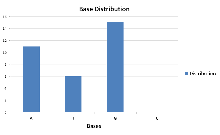
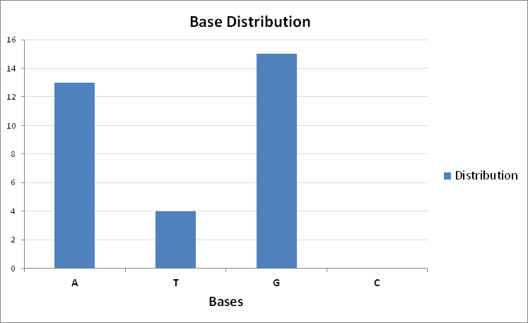
The predicted G base is the correct one. Below is the prediction of base distribution across the subsequences:
Figure 10: The prediction of base distribution across the subsequences of sequence `CACCCAATTGTGGTTGTGCAGCCAGATGCCTG`.
Thus the encoder was able to correctly predict the missing bases that needed to fill the gap:
CACCCAATTGTGGTTGTGCAGCCAGATGCCT[GG]ACAGAGGA
These results look promising! In the next section we will dive a bit deeper on what the model actually learned from the language of a genomic sequence.
What has the model learned? Diving Deeper Into the DNA Encoder Model
PyTorch has made it easy to look inside the model to determine what the DNA embeddings have learned from the genomic sequence through optimization via backpropagation:
# The following function will augment the DNAEncoder class
class DNAEncoder(nn.Module):
def get_sequence_embedding(self, embedded_sequence_index ):
return self.dna_embedding_table( embedded_sequence_index )
With this code we can extract the embedding table and frequency distribution of subsequences within the genome:
# Produce the subsequence genomic frequency distribution
alphabet_frequency = {}
for substring in dna_vocabulary:
index = -1
count = 0
while True:
index = genome.find( substring, index + 1, len(genome) )
if index > -1:
count = count + 1
else:
alphabet_frequency[ substring ] = count
break
embedding_header_file = open( r"embeddings_header.csv", "w+" )
embedding_file = open( r"embeddings.csv", "w+" )
alphabet_frequency_file = open( r"alphabet_frequency.csv", "w+" )
# Store the subsequence genomic frequency distribution to a file
for substring in alphabet_frequency:
alphabet_frequency_file.write( substring + ', ' +
str(alphabet_frequency[ substring ]) + '\n' )
alphabet_frequency_file.flush()
alphabet_frequency_file.close()
# Extract the embeddings of all subsequences, and
# store the embeddings to a file
for index in range( 0, len(dna_vocabulary) ):
embedding = model.get_sequence_embedding( torch.tensor( index ) )
list_of_floats = embedding.tolist()
embeddings_as_string = ''
embeddings_as_string = str( list_of_floats[0] )
for i in range(1, len(list_of_floats)):
embeddings_as_string = embeddings_as_string + \
", " + str( list_of_floats[i] )
embedding_file.write( embeddings_as_string + '\n' )
embedding_header_file.write( dna_vocabulary[index] + '\n' )
embedding_header_file.flush()
embedding_header_file.close()
embedding_file.flush()
embedding_file.close()
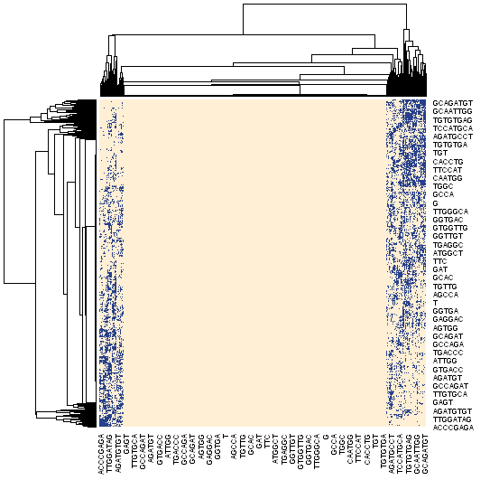
Given the embedding vectors of substrings we can perform the dot product of the embedding table to itself via the following:
This will produce the $|Sequence| \times |Sequence|$ matrix highlighting the pairwise subsequence affinity each other. This can be visualized as a heatmap:
Figure 11: The pairwise affinity of the genomic embeddings given their dot product shown as a heatmap.
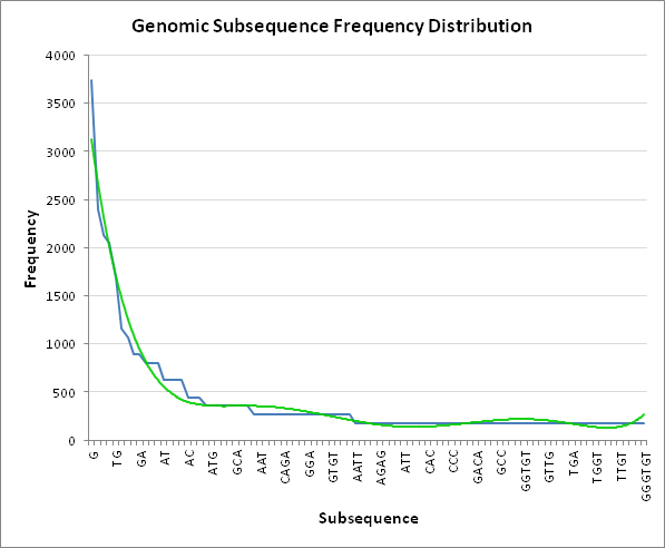
One noteable feature within the heatmap that jumps out is the emphasis on longer sequences, which makes sense as shorter sequences should have higher frequency, thus more entropy. We could peek at the distribution of the most frequent subsequences, which might give us some insight into their shared properties:
Figure 11: The distribution of subsequence frequencies across the genome, along with an overlay of the interpolated (green) trendline.
We can begin to see that the most frequent subsequences are naturally biased towards the more shorter sequences, which confirms that the embedding is weighted via backpropagation more towards the longer, less frequent subsequences. This naturally will shift the information towards the longer sequences, thus becoming more selective with predicting the next base, as supported by the highest attention for a given a subsequence.
There is more analysis in the works with which this report will be updated, but I hope this provides an overview of how using only the encoder of a transformer, one can fill in sequence gaps based on a model trained with the language of a genomic sequence.