ShallowVariant
This is a blog to illustrate the ideas of a neural network through a simplified variant caller named ShallowVariant.
In the previous blog we discussed how a neural network works. Here we will build a simpler variation of Google’s DeepVariant
Downloading the Data
The first step is to download the necessary files:
-
The first file we will download are the alignment files (BAM and BAI) for chromosome 20 of sample NA12878 (phase 3) from the 1000 Genomes dataset.
Sample NA12878 (1000 Genomes phase 3): https://ftp.1000genomes.ebi.ac.uk/vol1/ftp/phase3/data/NA12878/alignment/ -
The next file we will download is the Human Genome assembly GRCh37 (specifically hs37d5), since that was the reference used for aligning the FASTQ sequences in generating the BAM file.
Human Genome assembly GRCh37 (hs37d5) reference: https://ftp.1000genomes.ebi.ac.uk/vol1/ftp/technical/reference/phase2_reference_assembly_sequence/
These two files are sufficient to get us started. Throughout this blog other commonly used bioinformatic tools will be utilized to keep the example simple.
Performing the Pileup to Generate Candidate Variants with Truth Values
The next step is to extract candidate variants from the BAM file, by performing a pileup. A pileup is an aligment (mapping) of reads to a reference. If there is a region of variation among the reads and reference, then these will become candidates. In our case we will use freebayes, but other tools like bcftools mpileup will also work. The idea is to focus on bi-allelic SNPs (just to keep the problem simple), which we can use to build a neural network to predict the genotype. Since a pileup provides the position, we would not need the bases, and can rely only on the reference and alternate allelic depths. These provide information regarding the number of reads that support the reference or alternate allele.
Thus our goal is to see if we can estimate the genotypes from just the reference and alternate allelic depths, and use the truth values
- Reference Counts
- Alternate Counts
- Genotype
Therefore, we will run the following two commands to generate the answers:
The output of ref_alt_gt_ad.txt will look something like this (for just the bi-allelic SNPs):
I do realize there are additional filtering criteria such as minium coverage, and base quality scores, but we want to keep this example simple to connect the big ideas together $\text{–}$ and not become lost in the details.
The next step is to prepare these values for training a machine learning model.
Defining the Input (Tensor) and Output Labels
Now that we have bcftools-processed candidates from the VCF file, let’s try to generate the input to a neural network. In our example, the machine learning framework we will use is PyTorch. For a neural network model in PyTorch, the standard input is a tensor.
Since we’ll be taking a simpler approach, we will base our genotype predictions based on the following ratio (the symbols $||$ just refer to count or cardinality):
\[genotype \; \propto \dfrac{|reference|}{|reference| + |alternate|}\]Regarding the output genotype labels, they would need to have some form of numerical class label in order to be computable. Thus let’s label $homozygous \; reference$, $heterozygous$, and $heterozygous \; alternate$ as $1$ through $3$ $\text{–}$ with missing or uncallable (./.) labeled as $0$:
\[./. \rightarrow 0\] \[0/0 \rightarrow 1\] \[0/1 \: or \: 1/0 \rightarrow 2\] \[1/1 \rightarrow 3\]Thus before going too deep, let’s plot these and visualize what the genotype classes look like:
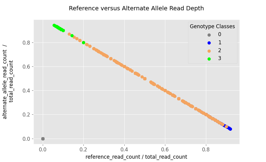
Based on the figure above, the genotype classes do not seem to separate very well, thus making the stratification by genotype-classes is not as clean. The fix would be to transform the space the data lives in, and a simple way would be to put them into $log$-$space$ by taking the $log_2$ of the two fractions:
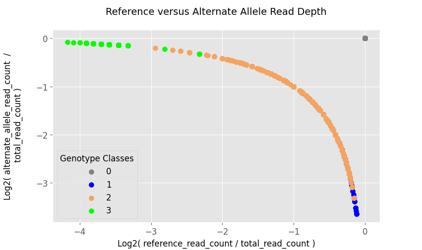
Now there seem to be better separation among the classes, allowing for the weights of the neural network model to be able to classify among the genotypes.
Loading and Processing the Data
Now we will be getting into the details of how to use PyTorch. We have a file called ref_alt_gt_ad.txt that we want to load. Let’s first start with a few variable definitions and helper functions.
The X and y vectors are instantiated as NumPy arrays $\text{–}$ with all zero values $\text{–}$ and having the following dimensions (shapes):
- X has dimensions 74732 rows x 2 columns, where two represents the reference and alternate allele
- y has dimensions 74732 elements to store the genotypes. You can think of it having one 74732 rows x 1 column, which is equivalent.
The values in X look as follows:
The values in y look as follows:
Next let’s define the function for loading the data:
Next we will define the multi-class neural network model.
Defining the MultiClass Neural Network Model
Let’s define the general network model for classifying for multiple genotype labels (i.e. more than two, or binary):
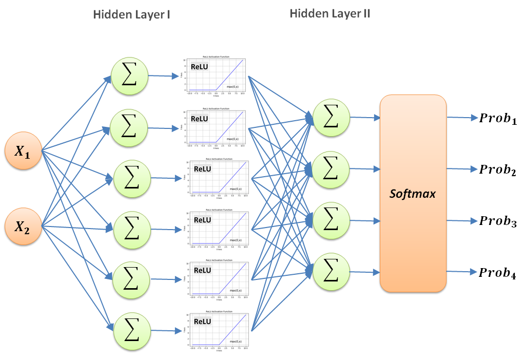
This is the same 2-layer neural network model you have seen before, but there are a few new additions. One of the most obvious additions is the increased number of nodes. We put more nodes at the beginning to get more details and the summarized the pertinent information by selecting only four nodes in the second hidden layer. That is a very common approach in neural network design to have more nodes initially and then focusing the results down the network to fewer and fewer ones.
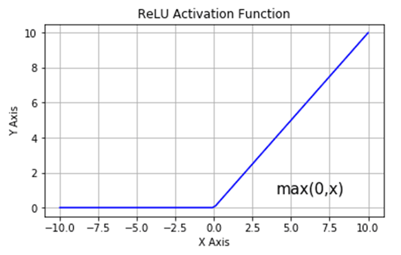
Another element in this network is the new activation function called $ReLU$, which stands for Rectified Linear Unit. Its behavior is by returning a value of $0$ for any input below 0, and returning back the input for anything higher than $0$. This is defined as follows:
\[f(x) = max(0, x) = \begin{cases} 0 & f(x) < 0 \\ x & f(x) \geq 0 \end{cases}\]Here x can represent complex interactions among multiple variables, which is transmitted to the next nodes of the model. The graph below shows the general behavior of the activation function:
The other characteristic that this model contains is the $softmax$ function, which turns a vector of values into probabilities (i.e. the sum of the values will then be equal to 1). The $softmax$ function is the following:
\[\sigma(\vec{z}) = \dfrac{e^{z_i}}{\Sigma^{K}_{j=1}e^{z_j}}\]Let’s begin to code the model up:
You will notice that we inherit the class torch.nn.Module, which is the base class for neural networks in PyTorch. Then we utilize the torch.nn.Linear class, which performs the linear transformations of $X \cdot W^T + bias$ calculations (where $W^T$ is the transpose of the weights).
One more important element when building a model is to randomize the data, and then use 80% for training the model and 20% for subsequently testing it. The testing step usually is not randomized. In our case we will randomly shuffle both stages, as the data loading methods in PyTorch will keep providing the same input for every round, which would not perform proper validation.
Let’s now train and test the neural network.
Implementing the MultiClass Neural Network Model
The first step is to define the model and a few initial variables that we will use:
If we print the values for train_size and test_size they will be 59785 and 14947, respectively.
The next we will generate the tensors. A tensor is the equivalent of the NumPy array, and is the standard data format in machine learning platforms, since it can remember additional parameters such as if it should reside on a GPU or CPU. Usually the shape (dimensions) of a tensor is defined as $(batch, channels, rows, columns)$, where channels are different data values of the rows and column, such as RGB (red, green, blue) values for an image. Batches are how many groups (sets) of the dimensions below $(channels, rows, columns)$ should be taken together in a calculation, such as for training or testing (validation).
Below are the instantiations of the tensors:
Next we will create dataset tensors to perform on-the-fly (lazy) data set reprentations for both training and testing. We will use dataloaders to shuffle and iterate over them. This nice tutorial provides a more friendly definition with examples.
Finally, let us define our model:
We will be training the model in batches, since we do not have enough computing power to train the whole dataset at once. Therefore with each training round (epoch), we take a batch and compare after training with how it performs against the expected (true) y values. Basically we compare the predicted $y$ with the true $y$, and based on their difference we optimize the model. With a bigger difference we optimize more, and vice versa if less. The $criterion$ measures how wrong our model performs, which is usually called the $loss \; (cost) \; function$. The loss will be used by the $optimizer \; function$ to adjust the model’s weights for the next round. Since we will be classifying across multiple classes, we will utilize the CrossEntropyLoss function:
The basic formula for cross entropy loss is the following:
\[Loss(\hat{y}, y) = - \Sigma^{K}_{k} y_k \cdot log( \hat{y}_k )\]Assuming the values of y are between 0 and 1, what the above formula calculates is the deviation among predicted outputs $\hat{y}$ in a batch, as compared to true (expected) values ($y$). What it really performs is the information (entropy, $H$) when having varied distributions. If the values are random, then these values will be high, and thus have a big loss (wrong result), requiring a larger shift in the weights of the neural network. Otherwise, they will stabilize and the loss will become minimal $\text{–}$ which is ideal $\text{–}$ making the model highly accurate in predicting the outcome.
Given the $loss \; function$ (or $criterion$), there needs to be another function to optimize based on the loss. For that we will use the Adam optimizer:
The Adam (Adaptive Moment Estimation) optimizerlr parameter is the initial learning rate to start with, meaning by how much to adjust the weights the first time when no gradients are available.
Now we are ready to begin to train the model.
Training the Model
Now we are ready to run through 10 epochs (rounds) to train the model, while checking on its loss and accuracy:
You might notice that we have a correct_count() function specified above. All that function performs is to determine how many of the predicted values y_pred match with the true values of y_batch. The contents of the function are the following:
While training the model, below is the output of each epoch:
| Epoch | Loss | Accuracy |
|---|---|---|
| 1 | 0.2682 | 97.07 % |
| 2 | 0.0249 | 98.19 % |
| 3 | 0.0203 | 99.26 % |
| 4 | 0.0179 | 99.26 % |
| 5 | 0.0141 | 99.30 % |
| 6 | 0.0137 | 99.36 % |
| 7 | 0.0124 | 99.39 % |
| 8 | 0.0121 | 99.42 % |
| 9 | 0.0119 | 99.41 % |
| 10 | 0.0117 | 99.45 % |
Below is a graph representing the above results:
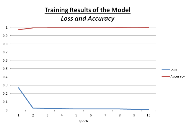
The general idea is that a model as it is being trained with each round will have a lower loss and become more accurate, which this is being exhibited here.
Testing the Model
Now we are ready to test how good our model behaves with testing data, which it has not seen before. Again we will go through 10 epochs (rounds) of testing, while checking on its loss and accuracy:
While testing the model, below is the output of each epoch:
| Epoch | Loss | Accuracy |
|---|---|---|
| 1 | 0.0095 | 99.61 % |
| 2 | 0.0105 | 99.61 % |
| 3 | 0.0110 | 99.61 % |
| 4 | 0.0093 | 99.61 % |
| 5 | 0.0119 | 99.61 % |
| 6 | 0.0106 | 99.61 % |
| 7 | 0.0108 | 99.61 % |
| 8 | 0.0096 | 99.61 % |
| 9 | 0.0094 | 99.61 % |
| 10 | 0.0106 | 99.61 % |
Below is a graph reprenting the above results:
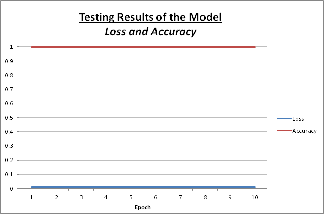
Based on the low loss and high accuracy the model performs fairly well.
Making Some Predictions
Now let us try to predict some genotypes. We will take the following sets of read counts for different positions:
| Position | Reference | Alternate |
|---|---|---|
| 1 | 10 | 1 |
| 2 | 10 | 10 |
| 3 | 1 | 10 |
We will need to take their fractions based on the total number of reads at each position, and then take the $log_2$ of each of those fractions:
The output result of the predictions is the following:
The results seem promising and will always get better with more data and more rounds of training.
One of the reasons I started this blog series is to unmystify what the models actually are performing internally. In the next section we will dive a bit deeper on what the model actually learned from the read depths to predict the genotype.
What has the model learned? Diving Deeper Into the Genotype Model
PyTorch has made it easy to look inside the model to determine what the weights have learned from the data:
The result is the following:
Mathematically these can be represented as the following:
Hidden Layer I (HL1)
\[\overrightarrow{\textbf{HL1}} = \begin{bmatrix} 0.9628 & 1.8207 \\ 0.1478 & 0.9089 \\ -1.2859 & -3.0906 \\ -2.5636 & 0.2988 \\ 1.6635 & 1.3060 \\ 1.4580 & 1.6511 \end{bmatrix} \cdot \begin{bmatrix} log_2( \dfrac{reference}{total} ) \\ log_2( \dfrac{alternate}{total} ) \end{bmatrix} +\] \[+ \begin{bmatrix} -1.6755 \; 2.9028 \; 2.2591 \; -0.6324 \; 1.6223 \; 1.8639 \end{bmatrix}\]Hidden Layer II (HL2)
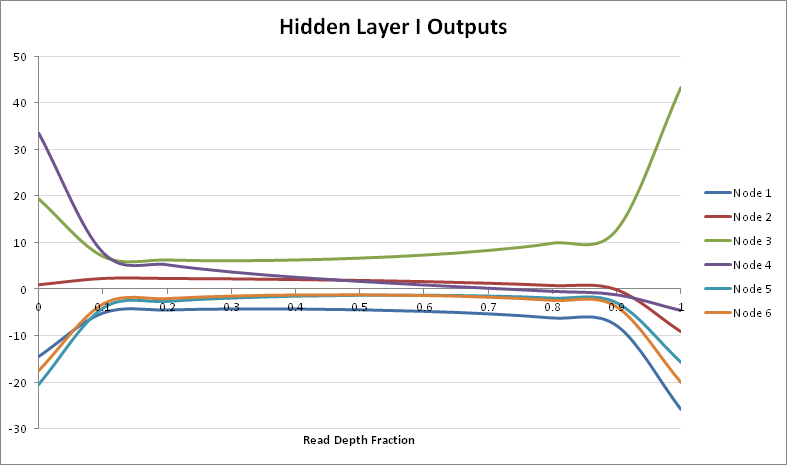
\[\overrightarrow{\textbf{HL2}} = \begin{bmatrix} -0.9532 & 1.7402 & -3.2636 & -2.2329 & 1.6347 & 1.9490 \\ -0.8620 & -2.1863 & 1.5901 & -2.7379 & -2.1378 & -1.5735 \\ -1.4391 & -0.5111 & 1.3885 & -0.3735 & -2.3134 & -1.8907 \\ 1.2431 & -2.6779 & -0.3130 & 2.1911 & -1.5693 & -1.8159 \end{bmatrix} \cdot ReLU( \overrightarrow{\textbf{HL1}} ) +\] \[+ \begin{bmatrix} 2.0075 & -1.6815 & -1.4783 & -1.9677 \end{bmatrix}\]Let us now try to inspect the effect of the weights across the range of read fractions. If we take a look at the outputs of Hidden Layer I, they are in the range from {$0.0001,…,0.9999$}. The node output distribution (for Hidden Layer I) across that range is as follows:
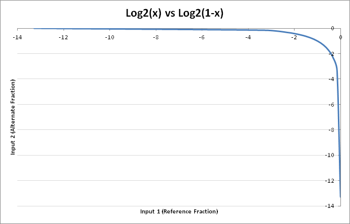
Another way the analysis can be viewed, is from the perspective of the binary contribution of the weights. The inputs are $(p, 1-p)$ where $p \in $ {$0,…,1$}, as is $1-p$. Thus given the log plot of the values, the highest contribution would be around $0.5$:
Thus the ReLU activation function will remove any negative contributions for upcoming layers of network. With that knowledge in mind, let’s explore which nodes actually have the most effect on predicting each genotype class:
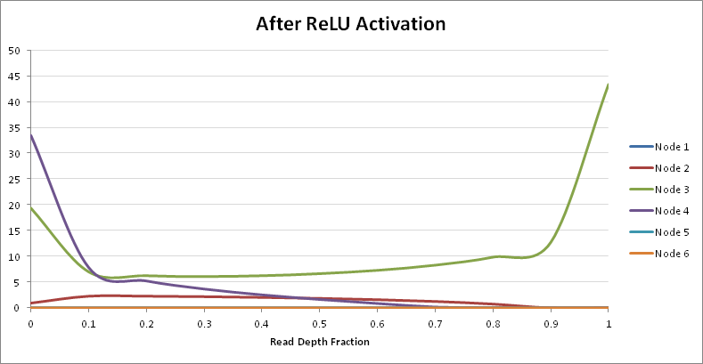
Given the above graph, it seems that only the weights of nodes 2, 3, and 4 of Hidden Layer I actually will have significant inpact in the separation of genotypes. With that knowledge, let’s explore the output of Hidden Layer II:
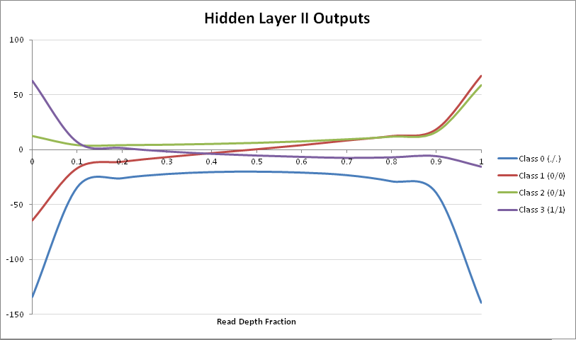
Based on the separation of genotype classes, only classes $1$ $(0/0)$, $2$ $(0/1)$ and $3$ $(1/1)$ perform separation among each other. Thus we can use class $1$ $(0/0)$ as a baseline to plot the other two against it, in order to determine separation of genotypes:
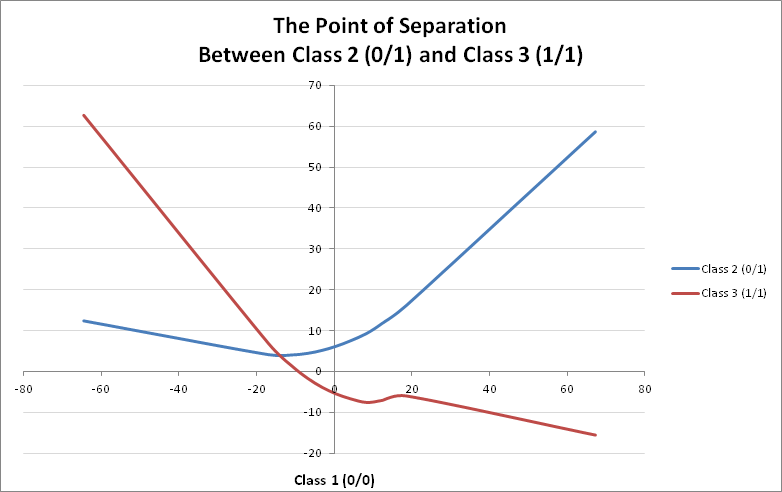
There is a clear point of intersection at around the value of $-14$ of class $1$ $(0/0)$, where a switch takes place among classes $2$ $(0/1)$ and $3$ $(1/1)$ $\text{–}$ emphasized by the weights.
There is more analysis in the works, with which this report will be updated, but I hope I gave you a overview of what neural network models learn and how genotype can be predicted just from the read depth.